Partitioning integers in factor
by Luca Di Sera
Why Integer Partitioning?
The last few months have been pretty stressful between university, searching for an interesting job ( which is absolutely the most stressful thing ), personal projects and, obviously, the whole COVID-19 situtation. I thus was looking for a breather, something that would distract myself and that I would be able to take less seriously than a personal project ( which, in the end, will stress me as I fight my unreachable perfection problem ).
I’ve decided to read Grune/Jacob’s Parsing Techniques. Now, in the book, the first parsing method that is encountered is that of Unger’s Parsers which requires all the k-compositions of the input string to execute.
To my surprise, it seems that there is no default way in factor to divide a sequence into k-compositions; or, at least, I was unable to find it neither by searching where I toughth it would be, namely, math.combinatorics, grouping or splitting; neither by a general search.
Thus, I decided to look a bit into the topic, which is mostly new to me ( I haven’t really done much combinatorics and I just know some small bits here and there that I learned when needed ).
Since we can build set-partitions/compositions from integer-partitions/compositions, I’ve decided to look into, specifically, integer-patitioning ( compositions can then be built from the partitions of the same number ).
What does it mean to partition an integer?
A partition of a positive integer is a multiset of positive integers which sum is . For example, is a partition of since .
| 1-partitions | 2-partitions | 3-partitions | 4-partitions | 5-partitions | 6-partitions | 7-partitions | 8-parttions |
|---|---|---|---|---|---|---|---|
| 8 | 7 + 1 | 6 + 1 + 1 | 5 + 1 + 1 + 1 | 4 + 1 + 1 + 1 + 1 | 3 + 1 + 1 + 1 + 1 + 1 | 2 + 1 + 1 + 1 + 1 + 1 + 1 | 1 + 1 + 1 + 1 + 1 + 1 + 1 + 1 |
| 6 + 2 | 5 + 2 + 1 | 4 + 2 + 1 + 1 | 3 + 2 + 1 + 1 + 1 + 1 | 2 + 2 + 1 + 1 + 1 + 1 | |||
| 5 + 3 | 4 + 2 + 2 | 3 + 2 + 2 + 1 | 2 + 2 + 2 + 1 + 1 | ||||
| 4 + 4 | 4 + 3 + 1 | 2 + 2 + 2 + 2 | |||||
| 3 + 3 + 2 | 3 + 3 + 1 + 1 |
We call an element of a partition a part. Thus, by of we will mean a partition of that has parts.
On a really basic level, this seems to be all there is to the definition of Integer Partitions.
On a more involved level, there seems to be a lot of cool knowledge related to Integer Partitions. One such bit that I encountered is the work done by mathematician Srinivasa Ramanujan( On which, by the way, there is a somewhat engaging movie ) on the partition function.
How are those partitions generated ?
There seems to be quite a few different sources on how to generate partitions. One of those sources seems to be from Knuth’s The Art Of Computer Programming which reminds me that I should really add the collection to my bookshelf as it is quite the unmatched reference ( which helped me a lot when looking at Random Number Generators ).
On a tangetially related note, the phrase “generating the partitions”, while not necessarily related to the generating function term, reminds me that I really want to read Wilf’s Generatingfunctionology but am currently unable as I don’t have the required mathematical knowledge, yet.
Of the methods I’ve found, I’ve decided to follow this paper by Katsuhisa Yamanaka,Shin-ichiro Kawano,Yosuke Kikuchi and Shin-ichi Nakano.
Partitions as a binary tree
This section is a summary of Sections [2,6] of the aforementioned paper. Much of the terminology and structure of the text comes from the paper and isn’t an original creation of mine.
The paper models the partitions of a positive integer as a binary tree ( called its family tree ).
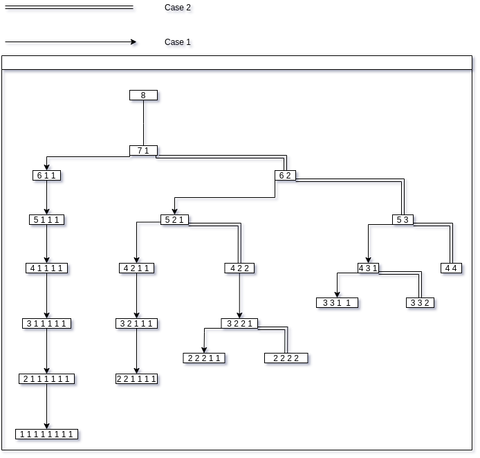 |
|---|
| Family tree for the positive number 8 |
Let be the set of all partitions of the positive integer .
From the paper, we define a partition as follows:
A partition is a monotonically decreasing sequence of positive integers , where holds, such that .
Each is called a part of .
Thus, for example:
- is a partition of four with four parts.
- is a partition of five with three parts.
- is a partition of six with three parts.
- cannot be a partition since .
The root of the binary tree is identified into the root partition, which is the partition that has a single part. The root partition is always a multiset with as its sole element.
There is then a single direct child to the root partition that has the form .
Given a partition that has at least two parts, there are two ways in which we can generate a new partition that is still ( thus each partition has at most two child and we can envision the partitions as a binary tree ). We call them and .
- ( In code, I call this a preserving child )[This terminology is not present in the paper]
We can generate from a partition by subtracting one from and adding one to . Thus, has the form .
- ( In code, I call this an expanding child )[This terminology is not present in the paper]
We can generate from a partition by subtracting one from and adding a one at the end. Thus, has form where .
Now, we can see that not every partition generates both or any valid partition or . For example, produces a preserving child which is not a partition as ( While not being a partition in our case, that is a composition of with parts ).
Each partition has either zero, one or two child. The paper identifies three cases:
-
- We have no child partition as holds in both and .
- and
- is not a partitition as holds in it.
- is a partition an thus we have one child.
- and . We consider two subcases:
- and
- is not a partition as holds in it.
- is a partition and thus we have one child.
- Otherwise
- Both and are partitions and thus we have two children.
- and
Thus, can be built by starting from the root partition, finding its direct child and then recursively generating the tree from there.
Let’s compute an example, we will find the partitions of .
- The root partition of is .
- The child of the root partition is .
- is of case 3.2, thus we have two children.
- is the child. It is a case 1 partition and thus has no child, making it a leaf of the tree.
- is the child. It is a case 2 partition and thus has an child.
- is the chld. It is a case 1 partition and thus has no child, making it a leaf of the tree.
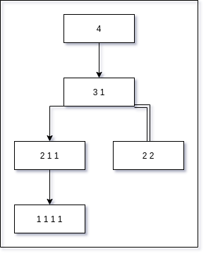 |
|---|
| Family tree for the positive number 4 |
Thus, the partitions of are , , , , .
Partitions with at most parts
If we want to only build the partitions of that have at most parts, we will call this set , we are able to do so by adding a restriction to the generation algorithm:
- If the currently inspected partition has an child and , we do not search the branch.
For example, the partitions of with at most parts can be generated as folllows:
- The root partition of is .
- The child of the root partition is .
- is of case 3.2, thus we have two children, but since we will not search the branch
- is the child. It is a case 1 partition and thus has no child, making it a leaf of the tree.
Partitions with exactly parts
We will call the set of partitions of with exactly parts, where holds, .
If there is a single, trivial partition of parts, i.e a multiset of ones.
In the case where , the paper shows that there is a bijection between and .
We can go from a partition to a partition , by subtracting one from each part of .
has exactly parts thus will have at most parts. Since we are removing one from each part, we will subtract from the sum of the partition, which is , and thus the new partition will have a sum of .
To go from a partition , with parts, to a partition , we will add one to each part of and then append ones to the resulting partition.
Since we are adding one to each part of , the new partition has a sum of . We then add ones and thus have a sum of .
Furthermore, we will have exactly parts.
Let’s look at an example, has the following elements, i.e all partitions of :
We can thus find the partitions of as follows:
- has part.
- is the result of adding one to each of its parts.
- is the result of appending ones to the new partition.
- has parts.
- is the result of adding one to each of its parts.
- is the result of appending ones to the new partition.
- has parts.
- is the result of adding one to each of its parts.
- is the result of appending ones to the new partition.
- has parts.
- is the result of adding one to each of its parts.
- is the result of appending ones to the new partition.
- has parts.
- is the result of adding one to each of its parts.
- is the result of appending ones to the new partition.
Thus the -partitions of are:
The paper has some more interesting sections about generating restricted partitions but I won’t cover them as they are not needed for the task at hand.
Implementing it in Factor
As the code is not particularly interesting, I won’t spend too much time explaining it.
generation as the atomic procedure
Generating from a procedure that generates is as easy as asking for . Further, from the paper we know that we can generate from .
If we consider the case where we have a procedure that generates , we could easily generate and by filtering the set. This case would be far from ideal, tough, as we would need to do a lot of unneded work ( and becomes big fast enough ).
If we, instead, are able to generate we could generate all partitions by applications and the same is true for generating . Again, this would require quite a bit of repeated or unneded work.
As such, I’ve started from a word that generates and built the other words from there.
I feel that this is a good middle ground. While we still incur in some overhead in not generating directly, it is negligible for our use case and simplifies the implementation.
Now, you will actually see that I completely disregarded performance here, as it was not the point of the exercise. The same is true for correctness and elegance. So talking about finding a good middle ground may feel a bit contradictory.
You may wonder, then, what did I not disregard. Uhm… probably nothing. The time I allotted for this exercise was small and thus I simply produced an “it works!” solution to better understand the domain.
Generating
The core of the generating procedure is the following, based on the code from the paper:
:: <=k-children ( partition k -- )
    partition ,
    partition has-an-expanding-child? [
        partition length k < [ partition expanding-child k <=k-children ] when
        partition has-a-preserving-child? [ partition preserving-child k <=k-children ] when
    ] when ;
This part is simple enough; if we consider the left child to be this basically describe a pre-order depth-first-search of our family tree.
we first collect the current partition. From , you can infer that the word is actually called trough make.
This wasn’t necessary and is a refuse from an initial implementation that was more contrived. Nonetheless, I think it might streamline the code a bit.
has-an-expanding-child is defined as follows:
: has-an-expanding-child? ( partition -- ? )
    first2 > ;
This check basically ensures that we are either in case 2 or 3 from the paper.
If you remember ( or check the first part of this article again ), if we have no child. In all other cases, we have an child.
Since we are generating , instead of directly recurring we have one more check to ensure that we actually want to generate that child that we know to be existing. If we do, i.e we are not working on a partition that has -parts, we recur and start descending the child-branch.
When we start to get back again, we check if we have an child and descend that branch.
has-a-preserving-child is defined as follows:
: has-a-preserving-child? ( partition -- ? )
    [ last2 [ > ] [ - 1 > ] 2bi ]
    [ length 2 > ]
    bi or and ;
We check if , thus putting us in the third case. Then we check that we are not in the first subcase such that we are in the general second subcase, which is the only case with an child.
The utility words expanding-child and preserving-child are defined as follows and are basically a one-to-one implementation of the generating procedure defined in the paper:
: expanding-child ( partition -- seq )
    unclip 1 - prefix 1 suffix ;

: preserving-child ( partition -- seq )
    unclip 1 - prefix unclip-last 1 + suffix ;
<=k-children is called from another word that provides the starting partition, i.e the child of the root partition, and calls make:
: root-child ( n -- partition )
    1 - 1 2array ;

: (<=k-partitions) ( n k -- partitions )
    [ root-child ] dip [ <=k-children ] { } make ;
As a last indirection, the actual public entry point, from which everything starts, is the following word:
: <=k-partitions ( n k -- partitions )
    [ [ [ 0 > ] both? ] [ drop 1array 1array ] [ { } ] smart-if* ]
    [
        [ [ 1 > ] bi@ and ]
        [ (<=k-partitions) append ]
        smart-when*
    ] 2bi ;
This is one of the ugliest parts of the code in my opinion and one of the first parts I would surely refactor.
Basically, we generate an empty-sequence in the case where the request is malformed, i.e or are not positive naturals. Otherwise, we generate a sequence containing the root partition and then dispatch to (<=k-partitions) and adding its result to our sequence.
This is all for generating .
A small example of it in action:
IN: scratchpad 8 4 <=k-partitions .
{
    { 8 }
    { 7 1 }
    { 6 1 1 }
    { 5 1 1 1 }
    { 6 2 }
    { 5 2 1 }
    { 4 2 1 1 }
    { 4 2 2 }
    { 3 2 2 1 }
    { 2 2 2 2 }
    { 5 3 }
    { 4 3 1 }
    { 3 3 1 1 }
    { 3 3 2 }
    { 4 4 }
}
IN: scratchpad 4 2 <=k-partitions .
{ { 4 } { 3 1 } { 2 2 } }
Generating
The word we implemented is already able to generate efficiently and providing a word for it is as trivial as follows:
: partitions ( n -- partitions )
    dup <=k-partitions ;
IN: scratchpad 12 partitions .
{
    { 12 }
    { 11 1 }
    { 10 1 1 }
    { 9 1 1 1 }
    { 8 1 1 1 1 }
    { 7 1 1 1 1 1 }
    { 6 1 1 1 1 1 1 }
    { 5 1 1 1 1 1 1 1 }
    { 4 1 1 1 1 1 1 1 1 }
    { 3 1 1 1 1 1 1 1 1 1 }
    { 2 1 1 1 1 1 1 1 1 1 1 }
    { 1 1 1 1 1 1 1 1 1 1 1 1 }
    { 10 2 }
    { 9 2 1 }
    { 8 2 1 1 }
    { 7 2 1 1 1 }
    { 6 2 1 1 1 1 }
    { 5 2 1 1 1 1 1 }
    { 4 2 1 1 1 1 1 1 }
    { 3 2 1 1 1 1 1 1 1 }
    { 2 2 1 1 1 1 1 1 1 1 }
    { 8 2 2 }
    { 7 2 2 1 }
    { 6 2 2 1 1 }
    { 5 2 2 1 1 1 }
    { 4 2 2 1 1 1 1 }
    { 3 2 2 1 1 1 1 1 }
    { 2 2 2 1 1 1 1 1 1 }
    { 6 2 2 2 }
    { 5 2 2 2 1 }
    { 4 2 2 2 1 1 }
    { 3 2 2 2 1 1 1 }
    { 2 2 2 2 1 1 1 1 }
    { 4 2 2 2 2 }
    { 3 2 2 2 2 1 }
    { 2 2 2 2 2 1 1 }
    { 2 2 2 2 2 2 }
    { 9 3 }
    { 8 3 1 }
    { 7 3 1 1 }
    { 6 3 1 1 1 }
    { 5 3 1 1 1 1 }
    { 4 3 1 1 1 1 1 }
    { 3 3 1 1 1 1 1 1 }
    { 7 3 2 }
    { 6 3 2 1 }
    { 5 3 2 1 1 }
    { 4 3 2 1 1 1 }
    { 3 3 2 1 1 1 1 }
    { 5 3 2 2 }
    { 4 3 2 2 1 }
    { 3 3 2 2 1 1 }
    { 3 3 2 2 2 }
    { 6 3 3 }
    { 5 3 3 1 }
    { 4 3 3 1 1 }
    { 3 3 3 1 1 1 }
    { 4 3 3 2 }
    { 3 3 3 2 1 }
    { 3 3 3 3 }
    { 8 4 }
    { 7 4 1 }
    { 6 4 1 1 }
    { 5 4 1 1 1 }
    { 4 4 1 1 1 1 }
    { 6 4 2 }
    { 5 4 2 1 }
    { 4 4 2 1 1 }
    { 4 4 2 2 }
    { 5 4 3 }
    { 4 4 3 1 }
    { 4 4 4 }
    { 7 5 }
    { 6 5 1 }
    { 5 5 1 1 }
    { 5 5 2 }
    { 6 6 }
}
IN: scratchpad 5 partitions .
{
    { 5 }
    { 4 1 }
    { 3 1 1 }
    { 2 1 1 1 }
    { 1 1 1 1 1 }
    { 3 2 }
    { 2 2 1 }
}
Generating
To generate we will thus use the method from the paper.
The conversion word is the following:
: <=k>=k ( partition k -- partition )
    [ [ [ 1 + ] map ] [ length ] bi ] dip swap - 1 <repetition> append ;
As per the paper we add to each part and then append ones to the end.
The entry point is the following:
: =k-partitions ( n k -- partitions )
    [ [ - ] keep <=k-partitions ]
    [ nip [ <=k>=k ] curry map ]
    2bi ;
Again, as per the paper we build and map it to .
For example:
IN: scratchpad 12 3 =k-partitions .
{
    { 10 1 1 }
    { 9 2 1 }
    { 8 2 2 }
    { 8 3 1 }
    { 7 3 2 }
    { 6 3 3 }
    { 7 4 1 }
    { 6 4 2 }
    { 5 4 3 }
    { 4 4 4 }
    { 6 5 1 }
    { 5 5 2 }
}
IN: scratchpad 7 6 =k-partitions .
{ { 2 1 1 1 1 1 } }
IN: scratchpad 240 1 =k-partitions .
{ { 240 } }
I find that those two words are particularly ugly and would probably look at refactoring them. I feel that I’m doing something unnecessary that could be shaved out. Maybe even something as simple as using lexical variables might make this better, like this:
:: =k-partitions ( n k -- partitions )
    n k - k <=k-partitions
    [ k <=k>=k ] map ;
When there is so much stack shuffling it may be a case of wrongly forming the interface so it may require some more work to become a decent implementation.
Intermezzo: A small test suite
While building the code I used a small test suite to check that I was going in the right direction.
! If either of the first two elements of the stack is 0 or less <=k-partitions produces the empty-sequence
{ t } [ 449944 0 <=k-partitions empty? ] unit-test
{ t } [ 0 567 <=k-partitions empty? ] unit-test

{ t } [ 449944 -235 <=k-partitions empty? ] unit-test
{ t } [ -1233 567 <=k-partitions empty? ] unit-test

! <=k-partitions constructs a sequence
{ t } [ 4 4 <=k-partitions sequence? ] unit-test

! The sequence produced by <=k-partitions contains sequences
{ t } [ 3 2 <=k-partitions [ sequence? ] all? ] unit-test

! The sequences contained in the sequence produced by <=k-partitions contain integers
{ t } [ 3 2 <=k-partitions flatten [ integer? ] all? ] unit-test

! The integers contained in the sequences that are elements of the sequence produced by <=k-partitions are greater than zero
{ t } [ 46 23 <=k-partitions flatten [ 0 > ] all? ] unit-test

! The sum of each sequence contained in the sequence produced by <=k-partitions is equal to the second element of the stack
{ t } [ 12 dup 7 <=k-partitions [ sum ] map [ = ] with all? ] unit-test

! The sequences contained in the sequence produced by <=k-partitions are monotonically decreasing
{ t } [ 14 9 <=k-partitions [ [ >= ] monotonic? ] all? ] unit-test

! The sequences contained in the sequence produced by <=k-partitions are of at most the head of the stack length
{ t } [ 13 11 [ <=k-partitions ] [ [ swap length >= ] curry all? ] bi ] unit-test

CONSTANT: <=k-partitions-test-data {
    { 8 2 {
         { 8 } { 7 1 } { 6 2 } { 5 3 } { 4 4 }
      } }
    { 4 3 {
        { 4 } { 3 1 } { 2 2 } { 2 1 1 }
      } }
    { 2 2 {
          { 2 } { 1 1 }
      } }
    { 3 8 {
          { 3 } { 2 1 } { 1 1 1 }
      } }
}

{ t } [ <=k-partitions-test-data [
            unclip-last [ first2 <=k-partitions ] dip [ natural-sort ] bi@ = ]
        [ and ] map-reduce
      ] unit-test

! If the first element of the stack is 0 or less partitions produces the empty-sequence
{ t } [ -23 partitions empty? ] unit-test
{ t } [ 0 partitions empty? ] unit-test

! partitions constructs a sequence
{ t } [ 5 partitions sequence? ] unit-test

! The sequence produced by partitions contains sequences
{ t } [ 2 partitions [ sequence? ] all? ] unit-test

! The sequences contained in the sequence produced by partitions contain integers
{ t } [ 7 partitions flatten [ integer? ] all? ] unit-test

! The integers contained in the sequences that are elements of the sequence produced by partitions are greater than zero
{ t } [ 9 partitions flatten [ 0 > ] all? ] unit-test

! The sum of each sequence contained in the sequence produced by partitions is equal to the head of the stack
{ t } [  7 dup partitions [ sum ] map [ = ] with all? ] unit-test

! The sequences contained in the sequence produced by partitions are monotonically decreasing
{ t } [ 2 partitions [ [ >= ] monotonic? ] all? ] unit-test

CONSTANT: partitions-test-data {
    { 8 {
          { 8 }
          { 7 1 } { 6 2 } { 5 3 } { 4 4 }
          { 6 1 1 } { 5 2 1 } { 4 2 2 } { 4 3 1 } { 3 3 2 }
          { 5 1 1 1 } { 4 2 1 1 } { 3 2 2 1 } { 2 2 2 2 } { 3 3 1 1 }
          { 4 1 1 1 1 } { 3 2 1 1 1 } { 2 2 2 1 1 }
          { 3 1 1 1 1 1 } { 2 2 1 1 1 1 }
          { 2 1 1 1 1 1 1 }
          { 1 1 1 1 1 1 1 1 }
      } }
    { 4 {
          { 4 }
          { 3 1 } { 2 2 }
          { 2 1 1 }
          { 1 1 1 1 }
      } }
    { 5 {
          { 5 }
          { 4 1 } { 3 2 }
          { 3 1 1 } { 2 2 1 }
          { 2 1 1 1 }
          { 1 1 1 1 1 }
      } }
}

{ t } [ partitions-test-data [
            first2 swap partitions [ natural-sort ] bi@ = ]
        [ and ] map-reduce
      ] unit-test


! If either of the first two elements of the stack is 0 or less =k-partitions produces the empty-sequence
{ t } [ 566060 0 =k-partitions empty? ] unit-test
{ t } [ 0 404030 =k-partitions empty? ] unit-test

{ t } [ 34 -235 =k-partitions empty? ] unit-test
{ t } [ -1233 345 =k-partitions empty? ] unit-test

! If the head of the 0 =k-partitions empty? ] unit-test

! =k-partitions constructs a sequence
{ t } [ 2 2 =k-partitions sequence? ] unit-test

! The sequence produced by =k-partitions contains sequences
{ t } [ 4 2 =k-partitions [ sequence? ] all? ] unit-test

! The sequences contained in the sequence produced by =k-partitions contain integers
{ t } [ 17 3 =k-partitions flatten [ integer? ] all? ] unit-test

! The integers contained in the sequences that are elements of the sequence produced by =k-partitions are greater than zero
{ t } [ 13 6 =k-partitions flatten [ 0 > ] all? ] unit-test

! The sum of each sequence contained in the sequence produced by =k-partitions is equal to the second element of the stack
{ t } [ 9 dup 6 =k-partitions [ sum ] map [ = ] with all? ] unit-test

! The sequences contained in the sequence produced by =k-partitions are monotonically decreasing
{ t } [ 22 12 =k-partitions [ [ >= ] monotonic? ] all? ] unit-test

! The sequences contained in the sequence produced by =k-partitions are exactly the head of the stack long
{ t } [ 7 2 [ =k-partitions ] [ [ swap length = ] curry all? ] bi ] unit-test

CONSTANT: =k-partitions-test-data {
    { 12 10 {
          { 3 1 1 1 1 1 1 1 1 1 } { 2 2 1 1 1 1 1 1 1 1 }
      } }
    { 7 2 {
          { 6 1 } { 5 2 } { 4 3 }
      } }
    { 6 3 {
          { 4 1 1 } { 3 2 1 } { 2 2 2 }
      } }
}

{ t } [ =k-partitions-test-data [
            unclip-last [ first2 =k-partitions ] dip [ natural-sort ] bi@ = ]
        [ and ] map-reduce
      ] unit-test
One thing that I was initially dabbling was testing the order of the produced sequence of partitions. I later decided to avoid enforcing a particular order ( even tough we do have a specific order in which we generate the partitions ) as I don’t think that such an invariant makes sense in this context.
While it was meant to be throwaway code, I still am not happy with it.
While I find it customary to check for type-correctness trough unit-testing in dynamic languages, I still dislike the fat it brings to a test suite.
Factor provides typed, so I would probably type the code and make the suite more lightweight in a more general context.
Most tests are repeated between the various partitions generating words. While I dislike this kind of repetition ( I would probably build some parameterized tests in this case ) I still feel that the fact that the words are built on one other is an implementation detail and should not creep to the public interface, thus requiring us to enforce the invariants, even if some are shared, for each word.
I can envision contexts in which the different algorithms are implemented for each word for some reason ( This actually points to the fact that instead of using <=k-partitions as an atomic procedure it may make sense to abstract the common parts of the algorithms and then implement the specific restrictions for each word ).
Obviously, the code itself is small and somewhat simple, but I still think that in a production environment a suite similar to this would be meaningless. It is true that in a production environment we would have ( well… it would really depend on where I would be working actually ) a good idea of what we were needing this for, what are the constraints and so on such that we may have a different or more defined execution context. Nonetheless, I still have the usual, malignant dilemma: Would I really do better than this?
Apart from the general dislike, I felt, again, the weight of the lack of a property-testing library in factor. I think that trying to tackle such a library might be an interesting project and wouldn’t mind trying it in the future.
But didn’t we need compositions?
As we said in the beginning, we actually need to compute the composition of an integer rather than its partitions.
The difference between the two is that partitions are unordered ( In the case of the paper we have an order constraint on them but that is not necessary ), such that is the same partition as , while compositions are ordered, thus and are different compositions.
It is trivial to see that compositions are simply the unique permutations of a partition. Thus, given , or we can find the corresponding set of compositions by mapping each element to its unique partitions.
Factor already provide the necessary code to so:
: compositions ( partitions -- compositions )
    [ all-permutations members ] [ append ] map-reduce ;
IN: scratchpad 4 partitions compositions .
{
    { 4 }
    { 3 1 }
    { 1 3 }
    { 2 1 1 }
    { 1 2 1 }
    { 1 1 2 }
    { 1 1 1 1 }
    { 2 2 }
}
IN: scratchpad 8 4 <=k-partitions compositions .
{
    { 8 }
    { 7 1 }
    { 1 7 }
    { 6 1 1 }
    { 1 6 1 }
    { 1 1 6 }
    { 5 1 1 1 }
    { 1 5 1 1 }
    { 1 1 5 1 }
    { 1 1 1 5 }
    { 6 2 }
    { 2 6 }
    { 5 2 1 }
    { 5 1 2 }
    { 2 5 1 }
    { 2 1 5 }
    { 1 5 2 }
    { 1 2 5 }
    { 4 2 1 1 }
    { 4 1 2 1 }
    { 4 1 1 2 }
    { 2 4 1 1 }
    { 2 1 4 1 }
    { 2 1 1 4 }
    { 1 4 2 1 }
    { 1 4 1 2 }
    { 1 2 4 1 }
    { 1 2 1 4 }
    { 1 1 4 2 }
    { 1 1 2 4 }
    { 4 2 2 }
    { 2 4 2 }
    { 2 2 4 }
    { 3 2 2 1 }
    { 3 2 1 2 }
    { 3 1 2 2 }
    { 2 3 2 1 }
    { 2 3 1 2 }
    { 2 2 3 1 }
    { 2 2 1 3 }
    { 2 1 3 2 }
    { 2 1 2 3 }
    { 1 3 2 2 }
    { 1 2 3 2 }
    { 1 2 2 3 }
    { 2 2 2 2 }
    { 5 3 }
    { 3 5 }
    { 4 3 1 }
    { 4 1 3 }
    { 3 4 1 }
    { 3 1 4 }
    { 1 4 3 }
    { 1 3 4 }
    { 3 3 1 1 }
    { 3 1 3 1 }
    { 3 1 1 3 }
    { 1 3 3 1 }
    { 1 3 1 3 }
    { 1 1 3 3 }
    { 3 3 2 }
    { 3 2 3 }
    { 2 3 3 }
    { 4 4 }
}
Uhm…okay that was easy. But didn’t we need to partition a sequence?
Why, yes that was our ultimate goal.
Again, we already have everything that we need at our disposal.
: split-compositions ( seq compositions -- seq )
    [ cum-sum split-indices but-last ] with map ;
Given a partition or a composition of of the form we can divide a sequence of length into parts by splitting the sequence at the cumulative sums, .
For example:
IN: scratchpad "pqrs" dup length partitions compositions split-compositions .
{
    { "pqrs" }
    { "pqr" "s" }
    { "p" "qrs" }
    { "pq" "r" "s" }
    { "p" "qr" "s" }
    { "p" "q" "rs" }
    { "p" "q" "r" "s" }
    { "pq" "rs" }
}
IN: scratchpad "pqrs" dup length 2 <=k-partitions split-compositions .
{ { "pqrs" } { "pqr" "s" } { "pq" "rs" } }
IN: scratchpad "(i+i)xi" dup length 3 =k-partitions compositions split-compositions .
{
    { "(i+i)" "x" "i" }
    { "(" "i+i)x" "i" }
    { "(" "i" "+i)xi" }
    { "(i+i" ")x" "i" }
    { "(i+i" ")" "xi" }
    { "(i" "+i)x" "i" }
    { "(i" "+" "i)xi" }
    { "(" "i+i)" "xi" }
    { "(" "i+" "i)xi" }
    { "(i+" "i)" "xi" }
    { "(i" "+i)" "xi" }
    { "(i" "+i" ")xi" }
    { "(i+" "i)x" "i" }
    { "(i+" "i" ")xi" }
    { "(" "i+i" ")xi" }
}
And that is exactly what we needed!
There is much more
The paper itself explores quite a few more interesting generating algorithms. Furthermore, for parsing grammars with -producing rules we would need to be able to generate partitions that have -parts and that is something that I may have to look at in the future.
The basic concept seems simple enough but I’ve really had a kick looking at this paper and would like to look at partitions a bit more. I will probably stop here, for now, as the objective was already reached and I have a plethora of exercises that I want to do.