Case Study 1 Delta Mush - Part 4

21 October 2018

by Luca Di Sera

Finding the time

Starting working has been a bit tough on my free time and, as such, on my study time. This post should have been done a long time ago ( and was actually completed a week before posting ) but having to commute about 2.5-3 hours a day for work has really reduced how fast I’m working on this deltaMush. Nonetheless I’m finally at a point where I think the new version is doably presentable. The main point of this version, and of this part of the case study, was the vectorization trough SIMD instructions of the deformer. This was actually done a bit of time ago, it took more time than it should because I decided to try and use a SOA structure, which has provided me with some interesteng challenges, and some other things. The code itself, again, isn’t really comparable with the previous version. Some of the things that have been done:

Vectorizing the code
Using a SOA structure for the data
Limiting the number of neighbours ( compromising )
Eliminating most of maya API code apart from getting and setting the points
Cleaning the code a bit

And so on… I really suggest you to look at the current code if you are interested in how it changed. As the main interest of this post is SIMD instructions we will have a small introduction on them and then look at the new code. But first…

Some Numbers, Again

There isn’t too much to say. As you can see from the graph 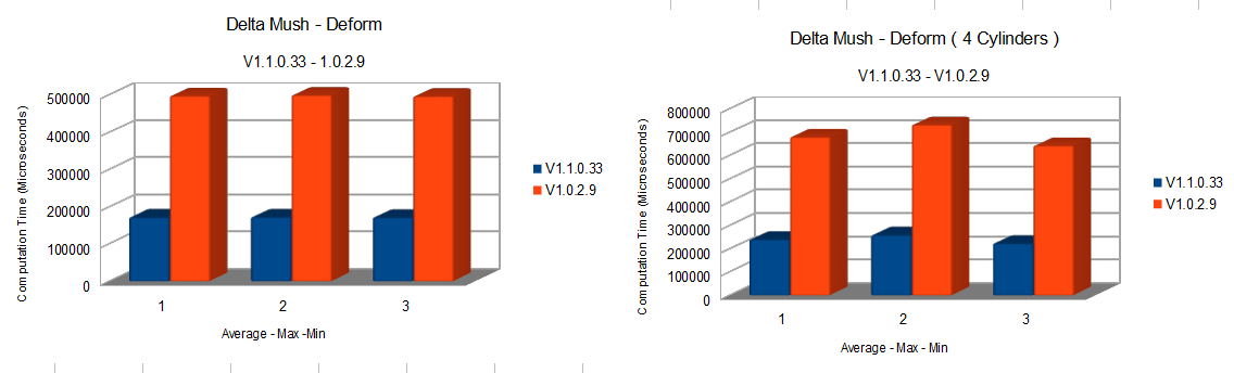final We are talking of about a 190% increase in performance. The ideal speedup would have been 4x but we haven’t shot too far from the target ( and considering that not all code was vectorizable we may have shoot more precisily than we think ). The main reason are AVX instructions but limiting the number of neighbours ( more on this later ) had a noticeable effect too. So much talk of SIMD, AVX, SOA and so on… But what are we talking about here?

A small introduction

Single Instruction, multiple data ( SIMD ) refers to a particular group of processor instructions which simultaneosly compute more than one piece of data. Exploiting data level parallelism we are able to compute, for example, the addition of 4 double to 4 double in a single instruction. We aren’t really talking about somehting new, as SIMD instruction predates the 21st century, and were popularized especially with Intel SSE/2/… in the early 2000s. For this project we are working with the AVX ( Advanced vector extension ) instruction set. This isn’t the most recent set but is what my current processor can support. By not using AVX2 or greater we are missing on some cool things like FMA ( Fused multiply add ) instructions or full lane permutes but nothing too daunting ( well, not having FMA is a bit daunting ). Now, we aren’t going as low level as using the instructions directly. We will help ourselves with some intrinsics.

Intrinsics basics

Intrisics are higher-level functions which wrap one or more of the processor instructions. They are accessible in C/C++ trough hedears file, in our case we will use “immintrin.h”. But what does AVX provides us with? Well first of all datatypes to work with SIMD instructions and a plethora of functions from mathematical operation like add, div or even sqrt, to shuffles, permutations, broadcasts, compare operators and much more. To understand the intrinsics syntax we have to understand its naming convention. Without understanding how things are named AVX code will look like unreadable, horrible magic. But I promise that understanding the following simple rules will make it a pleasure to read ( maybe not a pleasure but surely doable ).

First of all, AVX provides us with datatypes and functions. They both follow a similar naming convention.

Datatypes

We have only a few main datatypes to work with:

__m128
__m128d
__m128i
__m256
__m256d *__m256i

Each type starts with two underscore, followed by an m. After that there is the bits length of the register we intend to use. AVX/AVX2 go up to 256 bits, but more modern CPUs that support AVX512 get access to ( who would’ve guessed it ) 512 wide registers. With 256 bits we can store 4 doubles, 8 float or a different number of integers, depending on the type, up to 32 chars, 16 shorts, 8 ints, 4 longs. As you might have guessed, the suffix in the naming specifies the type of data we are working with.

No suffix means we are working with floats
d suffix means we are working with doubles
i suffix means we are working with integer-types and supports chars, shorts, ints and longs both signed and unsigned As you see, they may seem like hieroglyphs at first but they are actually pretty meaningful and expressive names when you know the convention behind them.

Functions

_mm256_add_pd()
_mm256_castps_pd()
_mm_add_ps()

Those are some intrinsics functions. A bit confusing I’m sure. Breaking it apart we have the following naming convention:

_mm<prefix>_<name>_<data_type>

_mm ( one underscore two ms instead of two underscores one m )
identifies the size of the vector returned by the function. It is empty for 128bits and 256 for the corresponding 256 bits vectors.
The of the operation we are going to execute ( add, sub, sqrt, cast, cvt... )
The data_type identifies the type of data we are working with. The pd in _mm256_add_pd means packed double precision and indicates we are working with doubles vectors. The possible suffix are constructed as follows:
The first one or two letters denotes if the data is (p)acked, (e)xtended-(p)acked or (s)calar. Scalar operations only works with the least-significant element ( bit 0-31 ) while packed operations work on multiple values in parallel.
The remaining letters denote the type, for example :
- s - single-precision floating-point ( floats )
- d - double-precision floating-point ( doubles )
- i128 - signed 128-bit integers
- i8/16/32/64 - signed integers vector containing 8/16/32/64 bits integers
- u8/16/32/64 - same as above but unsigned

E.G - _mm256_avg_epu16 Here we can understand, from just the function name that it returns a 256 bit vector which is of type __m256i. We can see that the function does something called avg. It is pretty explicative that avg is going to be average and so this function average its input. It won’t always be this clear tough. And we can see that this function works with extended-packed unsigned integers of 16 bit lenght.

Load…

We have functions that initialize the members of a vector directly ( for example _mm256_set1_pd(a) that sets all members to the one value that is passed ) and they are great. But, usually, we’d like to work with data we have in memory ( usually in a contiguous fashion ). That is done trough loads and stores.

__m256d _mm256_load_pd(double const * mem_addr)

This is the basic aligned load for 256 double vector. It literally loads the next 256 bit of memory from mem_addr as doubles and stores them in a __m256d that is returned. For example:

#include <immintrin.h>

int main() {
	double values[8]{ 1.0, 2.0, 3.0, 4.0, 5.0, 6.0, 7.0, 8.0 };

	// valuesVector will contain the values [ 3.0, 4.0, 5.0, 6.0 ] 
	__m256d valuesVector{ _mm256_load_pd(&values[2]) };
}

Now, this is the simplest load. We have other type of loads.

Unaligned loads ( _mm256_loadu_pd )
Mask loads ( _mm256_maskload_pd ). Mask loads get a second parameter that acts as a mask and is an integer vector of the size of the returned vector ( so __m256i for example ). Every element of the mask vector that has the highest bit as zero ( positive numbers ) sets the corresponding element in the returning vector to zero instead of loading it. Otherwise, if the highest bit is one ( negative numbers ) it reads the value from the mem_addr. A small example as it can be a bit confusing:

#include <immintrin.h>

int main() {
	float values[8]{ 1.0, 2.0, 3.0, 4.0, 5.0, 6.0, 7.0, 8.0 };

	// Negative values will be read from memory while positive addresses will be set to zero
	__m256i maskVector = _mm256_setr_epi32(1, -1, -1, -1, 1, -1, -1, 1);
	__m256 maskedVector = _mm256_maskload_ps(&values, maskVector);
	// maskedVector contains { 0.0, 2.0, 3.0, 4.0, 0.0, 6.0, 7.0, 0.0 } 
	
}

… modify and store

Now, after modifying our data, we need a way to get it back to our memory addresses. This is done trough stores functions. Store mostly mirrors loads, they get a mem_addr and a vector but instead of loading the memory into the vector they move the memory from the vector to the specified address. As with loads you have the possibility of masking the store.

For example, let’s say we have the following snippet we want to vetorize in a as straightforward-as-possible way:

int main() {
	float values[8]{ 1.0, 2.0, 3.0, 4.0, 5.0, 6.0, 7.0, 8.0 };
	float values2[8]{ 8.0, 7.0, 6.0, 5.0, 4.0, 3.0, 2.0 , 1.0 };
	float result[8]{};

	for (int i = 0; i < 8; ++i) {
		result[i] = (values[i] * values2[i]) + values[i];
	}

	for (int i = 0; i < 8; ++i) {
		std::cout << result[i] << std::endl;
	}

	std::cin.get();
}

This is pretty simple, we have to load our data, multiply and sum it and then store it back in result. This becomes something like this:

int main() {
	float values[8]{ 1.0, 2.0, 3.0, 4.0, 5.0, 6.0, 7.0, 8.0 };
	float values2[8]{ 8.0, 7.0, 6.0, 5.0, 4.0, 3.0, 2.0 , 1.0 };
	float result[8]{};

	__m256 valuesVector{ _mm256_load_ps(&values[0]) };
	__m256 valuesVector2{ _mm256_load_ps(&values2[0]) };

	__m256 intermediateVector{ _mm256_mul_ps(valuesVector, valuesVector2) };
	__m256 resultVector{ _mm256_add_ps(intermediateVector, valuesVector) };

	_mm256_store_ps(&result[0], resultVector);

	for (int i = 0; i < 8; ++i) {
		std::cout << result[i] << std::endl;
	}

	std::cin.get();
}

Simple as that. If we were to run this operation a big number of times we would already see a big improvement in computations time, however simple it is. If we had AVX2 we could do even better with FMA cutting the intermediate operation and multiplying and adding in one operation.

This are the basics of what intrinsics offers you. There is a world out there so I advise you to go and explore as it is quite the interesting world ( you can check the end of this post for some interesting resources ). Returning to our case-study, there is one more interesting thing to keep in mind…

SOA vs AOS

Let’s say we wanted to vectorize the following operation on vectors:

MVectorArray vectors{ 40u, MVector::one };
MVectorArray vectors2{ 40u, MVector::one };

MVectorArray sums{40u};

for (int i = 0; i < 40; ++i) {
	sums[i] = vectors[i] + vectors2[i];
}

Now this snippet too, is pretty straightforward, we could try something like this:

MVectorArray vectors{ 40u, MVector::one };
MVectorArray vectors2{ 40u, MVector::one };

MVectorArray sums{40u};

for (int i = 0; i < 40; ++i) {
	__m256d vector1{ _mm256_maskload_pd(&vectors[i].x, _mm256_setr_epi64x(-1ll, -1ll, -1ll, 1ll)) };
	__m256d vector2{ _mm256_maskload_pd(&vectors2[i].x, _mm256_setr_epi64x(-1ll, -1ll, -1ll, 1ll)) };
	__m256d result{ _mm256_add_pd(vector1, vector2) };

	_mm256_maskstore_pd(&sums[i].x, _mm256_setr_epi64x(-1ll, -1ll, -1ll, 1ll), result);
}

We could probably see some improvements with this version but there is a BIG problem: we are not utilizing our vector to the full. In fact, we waste a good 64 bits for registry and do only one sum at the time ( like the scalar version ). Our loads and stores are heavy too, so we have this little overhead for not much. This is happening because our data is layed out in a way that it is not easily parallelizable. Intrinsics are fast, that is sure, but what they really offer is parallel evaluation and we better use that to the fullest!

But what would our data layout look like to maximize our parallel capabilities ? SOA, what else!

Now, I’ve used this acronym a few times already and you’re probably scrathcing your head thinking about what its meaning could be. The way our data is usually layed out is called AOS ( Array Of Structure ). We are all familiar with this type of layout that may look something like this:

aos

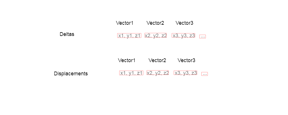
As we’ve seen, this isn’t ideal if we want to parallelize our vector operations. A better way to organize our data is called SOA ( Structure of Array ).

soa

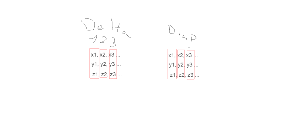
With a SOA layout we organize our data by components so that they are in a contiguos memory space. Our vectors are now indicized on multiple arrays that compose our structure. As you can easily guess this means we can load and compute more than one at a time directly.

for (int i = 0; i < 40; i += 4) {
		__m256d xVec1{ _mm256_load_pd(&x1) };
		__m256d yVec1{ _mm256_load_pd(&y1) };
		__m256d zVec1{ _mm256_load_pd(&z1) };

		__m256d xVec2{ _mm256_load_pd(&x2) };
		__m256d yVec2{ _mm256_load_pd(&y2) };
		__m256d zVec2{ _mm256_load_pd(&z2) };

		__m256d resX{ _mm256_add_pd(xVec1, xVec2) };
		__m256d resY{ _mm256_add_pd(yVec1, yVec2) };
		__m256d resZ{ _mm256_add_pd(zVec1, zVec2) };

With this we cut our iterations number by computing 4 vectors addition at once and we utilize all of our memory efficiently. This is the gist of it.

Usually you have two options.

Shuffling data on the fly to transform AOS loaded data into SOA form
Arrange or transform your data into SOA form and then transform it back if needed.

For the deltaMush code I decided to go full SOA as I did a big vectorization. Practically, I get the points positions, transform it to SOA, operate on the data and then converting back to AOS to store them. Now, converting data back and forth has a cost. But in our case this is more than ammortized by the time we save, especially because we have to convert from and to a single MPointArray only twice per computation ( four if the initialization has to be done ). Those are the functions I’m calling to convert back-and-forth:

// Copyright 2018 Luca Di Sera
//		Contact: disera.luca@gmail.com
//				 https://github.com/diseraluca
//				 https://www.linkedin.com/in/luca-di-sera-200023167
//
// This code is licensed under the MIT License. 
// More informations can be found in the LICENSE file in the root folder of this repository
//
//
// File : MPointArrayUtils.h
//
// The MPointArrayUtils namespace provides some utility functions for the deltaMush deformer.
// In particular the functions needed to move a MPointArray to SOA Form and back to an MPointArray.

#pragma once

#include <maya/MPointArray.h>
#include <immintrin.h>

namespace MPointArrayUtils {
	inline void decomposePointArray(MPointArray & points, double * out_x, double * out_y, double * out_z, unsigned int vertexCount)
	{
		double* pointsPtr{ &points[0][0] };

		for (unsigned int vertexIndex{ 0 }; vertexIndex < vertexCount; vertexIndex += 4, out_x += 4, out_y += 4, out_z += 4, pointsPtr += 16) {
			__m256d xx = _mm256_setr_pd(pointsPtr[0], pointsPtr[0 + 4], pointsPtr[0 + 8], pointsPtr[0 + 12]);
			__m256d yy = _mm256_setr_pd(pointsPtr[1], pointsPtr[1 + 4], pointsPtr[1 + 8], pointsPtr[1 + 12]);
			__m256d zz = _mm256_setr_pd(pointsPtr[2], pointsPtr[2 + 4], pointsPtr[2 + 8], pointsPtr[2 + 12]);

			_mm256_store_pd(out_x, xx);
			_mm256_store_pd(out_y, yy);
			_mm256_store_pd(out_z, zz);
		}
	}

	inline void composePointArray(double * x, double * y, double * z, MPointArray & out_points, unsigned int vertexCount)
	{
		double* pointsPtr{ &out_points[0][0] };

		for (unsigned int vertexIndex{ 0 }; vertexIndex < vertexCount; ++vertexIndex, ++x, ++y, ++z, pointsPtr += 4) {
			pointsPtr[0] = x[0];
			pointsPtr[1] = y[0];
			pointsPtr[2] = z[0];
			pointsPtr[3] = 1.0;
		}
	}
}

Furthermore, by using a memory layout that isn’t compatible with maya types I had to go-by without them. Fortunately, our data form is just a series of arrays but since the code was becoming unreadable I wrapped some common code in two utility-types :

// Copyright 2018 Luca Di Sera
//		Contact: disera.luca@gmail.com
//				 https://github.com/diseraluca
//				 https://www.linkedin.com/in/luca-di-sera-200023167
//
// This code is licensed under the MIT License. 
// More informations can be found in the LICENSE file in the root folder of this repository
//
//
// File : ComponentVector256d.h
//
// ComponentVector256d is an helper class for the deltaMush deformer aimed to improve code readability.
// It provides an interface for SOA Vectors that can contain and process 4 doubles at once.

#pragma once

#include <immintrin.h>

class ComponentVector256d {
public:

	/// Constructors
	inline ComponentVector256d() : x(_mm256_setzero_pd()), y(_mm256_setzero_pd()), z(_mm256_setzero_pd()) {}
	inline ComponentVector256d(const __m256d xx, const __m256d yy, const __m256d zz) : x(xx), y(yy), z(zz) {}
	inline ComponentVector256d(const double* xx, const double* yy, const double* zz) : x(_mm256_load_pd(xx)), y(_mm256_load_pd(yy)), z(_mm256_load_pd(zz)) {}

	// Set the components of the vector to the specified vectors
	inline void set(const __m256d xx, const __m256d yy, const __m256d zz) {
		x = xx;
		y = yy;
		z = zz;
	}

	// Set the components of the vector to zero
	inline void setZero() { 
		x = _mm256_setzero_pd();
		y = _mm256_setzero_pd();
		z = _mm256_setzero_pd();
	}

	// Return a vector containing the lengths of the contained vectors calculated as sqrt( x^2 + y^2 + z^2)
	inline __m256d length() const { return _mm256_sqrt_pd(_mm256_add_pd(_mm256_mul_pd(x, x), _mm256_add_pd(_mm256_mul_pd(y, y), _mm256_mul_pd(z, z)))); }

	// In-place normalization of the contained vectors
	inline void normalize() {
		__m256d factor{ _mm256_div_pd(_mm256_set1_pd(1.0), this->length()) };

		*(this) *= factor;
	}

	// Matrix - vector product where this is treated as an Nx3 matrix row
	inline __m256d asMatrixRowProduct(const ComponentVector256d& vector ) const {
		return _mm256_add_pd(_mm256_add_pd(_mm256_mul_pd(this->x, vector.x), _mm256_mul_pd(this->y, vector.y)), _mm256_mul_pd(this->z, vector.z));
	}

	inline void store(double* out_x, double* out_y, double* out_z) const {
		_mm256_store_pd(out_x, x);
		_mm256_store_pd(out_y, y);
		_mm256_store_pd(out_z, z);
	}

	/// ComponentVector256d - ComponentVector256d operators
	inline ComponentVector256d operator+(const ComponentVector256d& other) const { return ComponentVector256d(_mm256_add_pd(x, other.x), _mm256_add_pd(y, other.y), _mm256_add_pd(z, other.z)); }
	inline ComponentVector256d& operator+=(const ComponentVector256d& other) {
		x = _mm256_add_pd(x, other.x);
		y = _mm256_add_pd(y, other.y);
		z = _mm256_add_pd(z, other.z);

		return *this;
	}

	inline ComponentVector256d operator-(const ComponentVector256d& other) const { return ComponentVector256d(_mm256_sub_pd(x, other.x), _mm256_sub_pd(y, other.y), _mm256_sub_pd(z, other.z)); }
	inline ComponentVector256d operator*(const ComponentVector256d& other) const { return ComponentVector256d(_mm256_mul_pd(x, other.x), _mm256_mul_pd(y, other.y), _mm256_mul_pd(z, other.z)); }

	// The cross product operator
	inline ComponentVector256d operator^(const ComponentVector256d& other) const {
		return ComponentVector256d(
			_mm256_sub_pd(_mm256_mul_pd(y, other.z), _mm256_mul_pd(z, other.y)),
			_mm256_sub_pd(_mm256_mul_pd(z, other.x), _mm256_mul_pd(x, other.z)),
			_mm256_sub_pd(_mm256_mul_pd(x, other.y), _mm256_mul_pd(y, other.x))
		);
	}

	/// ComponentVector256d - __m256d operators
	inline ComponentVector256d operator*(const __m256d multiplier) const { return ComponentVector256d(_mm256_mul_pd(x, multiplier), _mm256_mul_pd(y, multiplier), _mm256_mul_pd(z, multiplier)); }
	inline ComponentVector256d& operator*=(const __m256d multiplier) { 
		x = _mm256_mul_pd(x, multiplier);
		y = _mm256_mul_pd(y, multiplier);
		z = _mm256_mul_pd(z, multiplier);

		return *this;
	}

public:
	__m256d x;
	__m256d y;
	__m256d z;
};

// Copyright 2018 Luca Di Sera
//		Contact: disera.luca@gmail.com
//				 https://github.com/diseraluca
//				 https://www.linkedin.com/in/luca-di-sera-200023167
//
// This code is licensed under the MIT License. 
// More informations can be found in the LICENSE file in the root folder of this repository
//
//
// File : ComponentVector256dMatrix3x3.h
//
// ComponentVector256dMatrix3x3 is an helper class for the deltaMush deformer aimed to improve code readability.
// It provides an interface to a 4-in-1 3x3 matrix that uses three ComponentVector256d as its rows.

#pragma once

#include "ComponentVector256d.h"

class ComponentVector256dMatrix3x3 {
public:
	/// Constructors
	inline ComponentVector256dMatrix3x3() :tangent(), normal(), binormal() {}

	// The product between a vector and the inverse of the matrix
	inline ComponentVector256d inverseProduct(const ComponentVector256d& vector) {
		__m256d length = _mm256_add_pd(_mm256_mul_pd(normal.x, normal.x), _mm256_add_pd(_mm256_mul_pd(normal.y, normal.y), _mm256_mul_pd(normal.z, normal.z)));
		__m256d factor = _mm256_div_pd(_mm256_set1_pd(1.0), length);

		normal *= factor;

		length = _mm256_add_pd(_mm256_mul_pd(binormal.x, binormal.x), _mm256_add_pd(_mm256_mul_pd(binormal.y, binormal.y), _mm256_mul_pd(binormal.z, binormal.z)));
		factor = _mm256_div_pd(_mm256_set1_pd(1.0), length);

		binormal *= factor;

		return ComponentVector256d(
			_mm256_add_pd(_mm256_add_pd(_mm256_mul_pd(tangent.x, vector.x), _mm256_mul_pd(normal.x, vector.y)), _mm256_mul_pd(binormal.x, vector.z)),
			_mm256_add_pd(_mm256_add_pd(_mm256_mul_pd(tangent.y, vector.x), _mm256_mul_pd(normal.y, vector.y)), _mm256_mul_pd(binormal.y, vector.z)),
			_mm256_add_pd(_mm256_add_pd(_mm256_mul_pd(tangent.z, vector.x), _mm256_mul_pd(normal.z, vector.y)), _mm256_mul_pd(binormal.z, vector.z))
		);
	}

	/// Matrix - Vector operators
	inline ComponentVector256d operator*(const ComponentVector256d& vector) {
		return ComponentVector256d(
			_mm256_add_pd(_mm256_add_pd(_mm256_mul_pd(this->tangent.x, vector.x), _mm256_mul_pd(this->tangent.y, vector.y)), _mm256_mul_pd(this->tangent.z, vector.z)),
			_mm256_add_pd(_mm256_add_pd(_mm256_mul_pd(this->normal.x, vector.x), _mm256_mul_pd(this->normal.y, vector.y)), _mm256_mul_pd(this->normal.z, vector.z)),
			_mm256_add_pd(_mm256_add_pd(_mm256_mul_pd(this->binormal.x, vector.x), _mm256_mul_pd(this->binormal.y, vector.y)), _mm256_mul_pd(this->binormal.z, vector.z))
		);
	}

public:
	ComponentVector256d tangent;
	ComponentVector256d normal;
	ComponentVector256d binormal;
};

They are tailor made to the code I wrote, provide only the methods I currently need, and aren’t geared towards a general use case. But they do their work, helping me with code readability at least a bit. For example, the following code:

for (unsigned int vertexIndex{ 0 }; vertexIndex < vertexCount; vertexIndex += 4, neighbourPtr += 12) {
			averageX = _mm256_setzero_pd();
			averageY = _mm256_setzero_pd();
			averageZ = _mm256_setzero_pd();

			for (unsigned int neighbourIndex{ 0 }; neighbourIndex < MAX_NEIGHBOURS; ++neighbourIndex, ++neighbourPtr) {
				__m256d neighboursX = _mm256_setr_pd(verticesCopyX[neighbourPtr[0]], verticesCopyX[neighbourPtr[0 + 4]], verticesCopyX[neighbourPtr[0 + 8]], verticesCopyX[neighbourPtr[0 + 12]]);
				__m256d neighboursY = _mm256_setr_pd(verticesCopyY[neighbourPtr[0]], verticesCopyY[neighbourPtr[0 + 4]], verticesCopyY[neighbourPtr[0 + 8]], verticesCopyY[neighbourPtr[0 + 12]]);
				__m256d neighboursZ = _mm256_setr_pd(verticesCopyZ[neighbourPtr[0]], verticesCopyZ[neighbourPtr[0 + 4]], verticesCopyZ[neighbourPtr[0 + 8]], verticesCopyZ[neighbourPtr[0 + 12]]);

				averageX = _mm256_add_pd(averageX, neighboursX);
				averageY = _mm256_add_pd(averageY, neighboursY);
				averageZ = _mm256_add_pd(averageZ, neighboursZ);
			}

			// Divides the accumulated vector to average it
			__m256d averageFactorVec = _mm256_set1_pd(AVERAGE_FACTOR);

			averageX = _mm256_mul_pd(averageX, averageFactorVec);
			averageY = _mm256_mul_pd(averageY, averageFactorVec);
			averageZ = _mm256_mul_pd(averageZ, averageFactorVec);

			__m256d verticesCopyXVector = _mm256_load_pd(verticesCopyX + vertexIndex);
			__m256d verticesCopyYVector = _mm256_load_pd(verticesCopyY + vertexIndex);
			__m256d verticesCopyZVector = _mm256_load_pd(verticesCopyZ + vertexIndex);

			averageX = _mm256_sub_pd(averageX, verticesCopyXVector);
			averageY = _mm256_sub_pd(averageY, verticesCopyYVector);
			averageZ = _mm256_sub_pd(averageZ, verticesCopyZVector);

			averageX = _mm256_mul_pd(averageX, weighVector);
			averageY = _mm256_mul_pd(averageY, weighVector);
			averageZ = _mm256_mul_pd(averageZ, weighVector);

			averageX = _mm256_add_pd(averageX, verticesCopyXVector);
			averageY = _mm256_add_pd(averageY, verticesCopyYVector);
			averageZ = _mm256_add_pd(averageZ, verticesCopyZVector);

			_mm256_store_pd(smoothedX + vertexIndex, averageX);
			_mm256_store_pd(smoothedY + vertexIndex, averageY);
			_mm256_store_pd(smoothedZ + vertexIndex, averageZ);
		}

becomes :

for (unsigned int vertexIndex{ 0 }; vertexIndex < vertexCount; vertexIndex += 4, neighbourPtr += 12) {
			average.setZero();

			for (unsigned int neighbourIndex{ 0 }; neighbourIndex < MAX_NEIGHBOURS; ++neighbourIndex, ++neighbourPtr) {
				ComponentVector256d neighbourPositions{
					_mm256_setr_pd(verticesCopyX[neighbourPtr[0]], verticesCopyX[neighbourPtr[0 + 4]], verticesCopyX[neighbourPtr[0 + 8]], verticesCopyX[neighbourPtr[0 + 12]]),
					_mm256_setr_pd(verticesCopyY[neighbourPtr[0]], verticesCopyY[neighbourPtr[0 + 4]], verticesCopyY[neighbourPtr[0 + 8]], verticesCopyY[neighbourPtr[0 + 12]]),
					_mm256_setr_pd(verticesCopyZ[neighbourPtr[0]], verticesCopyZ[neighbourPtr[0 + 4]], verticesCopyZ[neighbourPtr[0 + 8]], verticesCopyZ[neighbourPtr[0 + 12]])
				};

				average += neighbourPositions;
			}

			// Divides the accumulated vector to average it
			__m256d averageFactorVec = _mm256_set1_pd(AVERAGE_FACTOR);
			average *= averageFactorVec;

			ComponentVector256d verticesCopyPositions{ verticesCopyX.data() + vertexIndex, verticesCopyY.data() + vertexIndex, verticesCopyZ.data() + vertexIndex };

			average = (average - verticesCopyPositions) * weighVector + verticesCopyPositions;
			average.store(smoothedX.data() + vertexIndex, smoothedY.data() + vertexIndex, smoothedZ.data() + vertexIndex);

		}

Which is a lot more readable.

Some other structural changes

One thing that is of note, before looking at a vectorization code example from the deformer, is that I decided to limit the number of neighbours for each vertex to a known, arbitrary number. In this case four. What does this imply? Well first of all, we are obviosly compromising here. We get so much, performance wise, as we save a lot of computations, like all the length() methods, we move some to compile time and we help the compiler a lot. But we lose a lot the other way too. As we are limiting the number of neighbours, we are obviosly approximating the smoothing. This is absurdly obvious on the test scenes I use, for example. As the caps of the cylinders have around 12 neighbours, using only 4 and considering how vertex IDs are set on the Cylinder primitive we have an big error on the central vertex that moves to one of the sides.

For this exercise this is more than okay, I’m not writing with a production level in mind. In a working environment usually you would have more than one version of this or have some flag to activate or deactivate this limit.

Other than that it should be noted that as we are now working with batches of four doubles at a time, some arrays had to be padded to simplify the code and avoid memory errors. You can see it from the new getNeighbours :

MStatus DeltaMush::getNeighbours(MObject & mesh, unsigned int vertexCount)
{
	neighbours.resize(paddedCount * MAX_NEIGHBOURS);
	std::fill(neighbours.begin(), neighbours.end(), 0.0);

	MItMeshVertex meshVtxIt{ mesh };
	MIntArray temporaryNeighbours{};
	int currentVertex{};
	for (unsigned int vertexIndex{ 0 }; vertexIndex < vertexCount; ++vertexIndex, meshVtxIt.next()) {
		meshVtxIt.getConnectedVertices(temporaryNeighbours);

		currentVertex = vertexIndex * MAX_NEIGHBOURS;
		if (temporaryNeighbours.length() >= MAX_NEIGHBOURS) {
			neighbours[currentVertex + 0] = temporaryNeighbours[0];
			neighbours[currentVertex + 1] = temporaryNeighbours[1];
			neighbours[currentVertex + 2] = temporaryNeighbours[2];
			neighbours[currentVertex + 3] = temporaryNeighbours[3];
		}
		else {
			for (unsigned int neighbourIndex{ 0 }; neighbourIndex < MAX_NEIGHBOURS; ++neighbourIndex) {
				if (neighbourIndex < temporaryNeighbours.length()) {
					neighbours[currentVertex + neighbourIndex] = temporaryNeighbours[neighbourIndex];
				}
				else {
					// With this we expect every vertex to have at least two neighbours
					neighbours[currentVertex + neighbourIndex] = neighbours[currentVertex + neighbourIndex - 2];
				}
			}
		}
	}

	return MStatus::kSuccess;
}

An example

Let’s work trough an example. We’ll use the apply delta part that is at the end of the chain. Let’s look at the previous version of the code:

MMatrix tangentSpaceMatrix{};
	double* tangentPtr{ &tangentSpaceMatrix.matrix[0][0] };
	double* normalPtr{ &tangentSpaceMatrix.matrix[1][0] };
	double* binormalPtr{ &tangentSpaceMatrix.matrix[2][0] };

	double* vertexPositionsPtr{ &meshVertexPositions[0].x };
	double *smoothedPositionsPtr{ &meshSmoothedPositions[0].x };
	double *resultPositionsPtr{ &resultPositions[0].x };
	
	double length{};
	double factor{};
	unsigned int neighbourIterations{};

	float envelopeValue{ block.inputValue(envelope).asFloat() };
	double deltaWeightValue{ block.inputValue(deltaWeight).asDouble() };

	for (int vertexIndex{ 0 }; vertexIndex < vertexCount; ++vertexIndex, resultPositionsPtr += 4, vertexPositionsPtr += 4) {
		// resetting the delta vector
		deltaPtr[0] = 0.0;
		deltaPtr[1] = 0.0;
		deltaPtr[2] = 0.0;

		neighbourIterations = neighbours[vertexIndex].length() - 1;
		for (unsigned int neighbourIndex{ 0 }; neighbourIndex < neighbourIterations; ++neighbourIndex) {

			// Calculate the vectors between the current vertex and two of its neighbours
			tangentPtr[0] = smoothedPositionsPtr[neighbours[vertexIndex][neighbourIndex] * 4] - smoothedPositionsPtr[vertexIndex * 4];
			tangentPtr[1] = smoothedPositionsPtr[neighbours[vertexIndex][neighbourIndex] * 4 + 1] - smoothedPositionsPtr[vertexIndex * 4 + 1];
			tangentPtr[2] = smoothedPositionsPtr[neighbours[vertexIndex][neighbourIndex] * 4 + 2] - smoothedPositionsPtr[vertexIndex * 4 + 2];

			normalPtr[0] = smoothedPositionsPtr[neighbours[vertexIndex][neighbourIndex + 1] * 4] - smoothedPositionsPtr[vertexIndex * 4];
			normalPtr[1] = smoothedPositionsPtr[neighbours[vertexIndex][neighbourIndex + 1] * 4 + 1] - smoothedPositionsPtr[vertexIndex * 4 + 1];
			normalPtr[2] = smoothedPositionsPtr[neighbours[vertexIndex][neighbourIndex + 1] * 4 + 2] - smoothedPositionsPtr[vertexIndex * 4 + 2];

			// Normalizes the two vectors.
			// Vector normalization is calculated as follows:
			// lenght of the vector -> sqrt(x*x + y*y + z*z)
		    // [x, y, z] / length
			length = std::sqrt(tangentPtr[0] * tangentPtr[0] + tangentPtr[1] * tangentPtr[1] + tangentPtr[2] * tangentPtr[2]);

			factor = 1.0 / length;
			tangentPtr[0] *= factor;
			tangentPtr[1] *= factor;
			tangentPtr[2] *= factor;

			length = std::sqrt(normalPtr[0] * normalPtr[0] + normalPtr[1] * normalPtr[1] + normalPtr[2] * normalPtr[2]);

			factor = 1.0 / length;
			normalPtr[0] *= factor;
			normalPtr[1] *= factor;
			normalPtr[2] *= factor;

			// Ensures  axis orthogonality through cross product.
			// Cross product is calculated in the following code as:
			// crossVector = [(y1 * z2 - z1 * y2), (z1 * x2 - x1 * z2), (x1 * y2 - y1 * x2)]
			binormalPtr[0] = tangentPtr[1] * normalPtr[2] - tangentPtr[2] * normalPtr[1];
			binormalPtr[1] = tangentPtr[2] * normalPtr[0] - tangentPtr[0] * normalPtr[2];
			binormalPtr[2] = tangentPtr[0] * normalPtr[1] - tangentPtr[1] * normalPtr[0];

			normalPtr[0] = tangentPtr[1] * binormalPtr[2] - tangentPtr[2] * binormalPtr[1];
			normalPtr[1] = tangentPtr[2] * binormalPtr[0] - tangentPtr[0] * binormalPtr[2];
			normalPtr[2] = tangentPtr[0] * binormalPtr[1] - tangentPtr[1] * binormalPtr[0];

			// Accumulate the displacement Vectors
			// TODO : Provide a custom matrix*vector implementation to remove the intermediate MVector and transform the MMatrix into a simpler double[4][4]
			MVector tangentSpaceDelta{ tangentSpaceMatrix * deltas[vertexIndex][neighbourIndex] };
			deltaPtr[0] += tangentSpaceDelta.x;
			deltaPtr[1] += tangentSpaceDelta.y;
			deltaPtr[2] += tangentSpaceDelta.z;
		}

		// Averaging the delta
		factor = (1.0 / neighbourIterations);
		deltaPtr[0] *= neighbourIterations;
		deltaPtr[1] *= neighbourIterations;
		deltaPtr[2] *= neighbourIterations;

		// Scaling the delta
		delta.normalize();
		deltaPtr[0] *= (deltaMagnitudes[vertexIndex] * deltaWeightValue);
		deltaPtr[1] *= (deltaMagnitudes[vertexIndex] * deltaWeightValue);
		deltaPtr[2] *= (deltaMagnitudes[vertexIndex] * deltaWeightValue);

		// Finding the final position
		resultPositionsPtr[0] = smoothedPositionsPtr[vertexIndex * 4] + deltaPtr[0];
		resultPositionsPtr[1] = smoothedPositionsPtr[vertexIndex * 4 + 1] + deltaPtr[1];
		resultPositionsPtr[2] = smoothedPositionsPtr[vertexIndex * 4 + 2] + deltaPtr[2];
		resultPositionsPtr[3] = 1.0;

		// We calculate the new definitive delta
		deltaPtr[0] = resultPositionsPtr[0] - vertexPositionsPtr[0];
		deltaPtr[1] = resultPositionsPtr[1] - vertexPositionsPtr[1];
		deltaPtr[2] = resultPositionsPtr[2] - vertexPositionsPtr[2];

		// Setting the weighted final position
		resultPositionsPtr[0] = vertexPositionsPtr[0] + (deltaPtr[0] * perVertexWeights[vertexIndex] * envelopeValue);
		resultPositionsPtr[1] = vertexPositionsPtr[1] + (deltaPtr[1] * perVertexWeights[vertexIndex] * envelopeValue);
		resultPositionsPtr[2] = vertexPositionsPtr[2] + (deltaPtr[2] * perVertexWeights[vertexIndex] * envelopeValue);
	}

	iterator.setAllPositions(resultPositions);

Before we modify the code, we should look at how our data is layed out currently. In the new version the data that comes to us is in SOA form. We have a few arrays that contains what we need. I layed it out visually in the next image :

incomingData

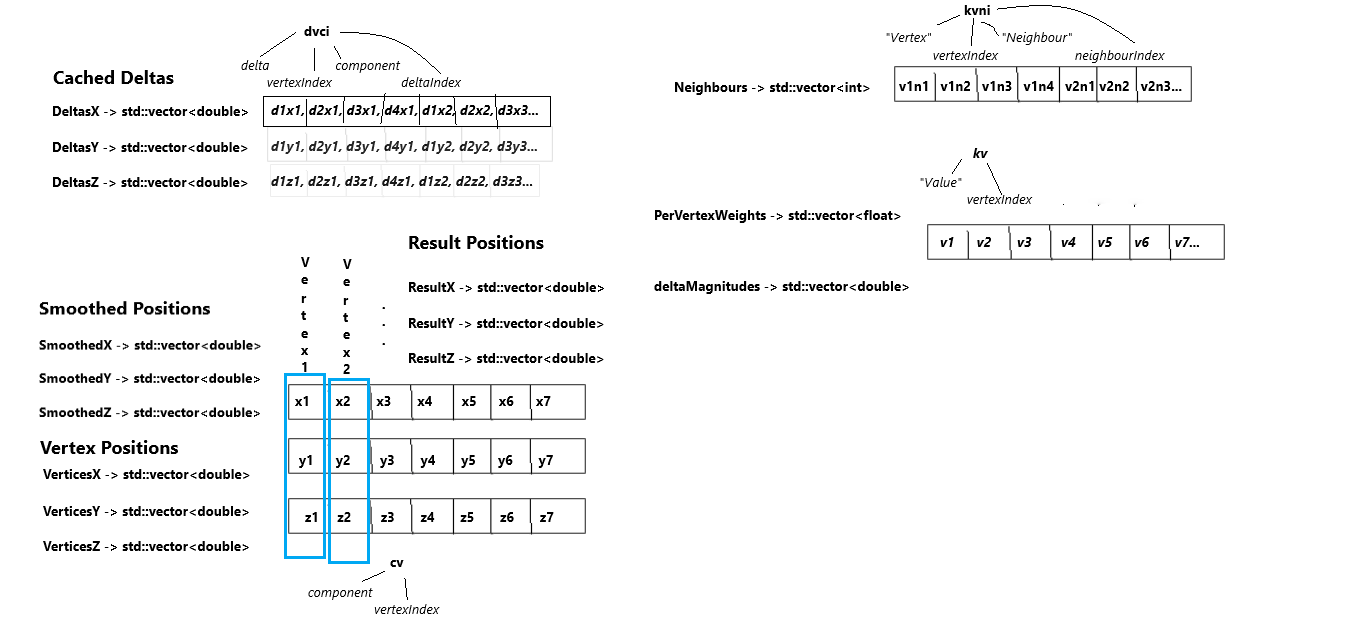
As you can see we have about three type of layouts:

Single array data like neighbours and deltaMagnitudes. Those are single arrays containing all the data with a value per vertex. Neighbors is a bit particular confronted to the other two as it contains multiple values for each vertex in linear order.

Component vectors like VertexPositions which are laid out on three arrays, one for each component. Each array contains one value for each vertex. With this form, we can index a specific vector through the 3 arrays, as they are all aligned so that the value in the first memory cell refers to the same vector on all arrays. CachedDeltas has three component arrays like vectors. It contains multiple values per vertex like Neighbours. The difference is that its data is interleaved so that we have the first delta for the first four vertexes consecutively followed by the second delta for the first four vertexes and so on.

Now that we know what and how are things coming to us let’s return to the code.

Cutting the iterations by 4

Let’s first think about our main loops.

for (int vertexIndex{ 0 }; vertexIndex < vertexCount; ++vertexIndex, resultPositionsPtr += 4, vertexPositionsPtr += 4) {
		// Things going on
		for (unsigned int neighbourIndex{ 0 }; neighbourIndex < neighbourIterations; ++neighbourIndex) {}
}

Now, the first thing we can see is that currently, as we are working with serial operations, we compute one vertex/delta per iterations and, as such, we have to iterate as much as there are vertexes.

Now, with how our data is laid out ( and with arrays always padded to be multiple of four and neighbors always 4 per-vertex ), working with doubles we can compute four values at once. This means our main loop will need to advance by four vertexes per iteration and our neighbor loop will still run the same number of iterations but will compute 4 deltas per iteration.

In code:

for (int vertexIndex{ 0 }; vertexIndex < vertexCount; vertexIndex += 4, neighbourPtr += 13) {
for (unsigned int neighbourIndex{ 0 }; neighbourIndex < DELTA_COUNT; ++neighbourIndex, ++neighbourPtr, deltaXPtr += 4, deltaYPtr += 4, deltaZPtr += 4)
}

Now, the way the variables state flows requires some explanation. Let’s start with how the neighbor works.

neighboursFlow

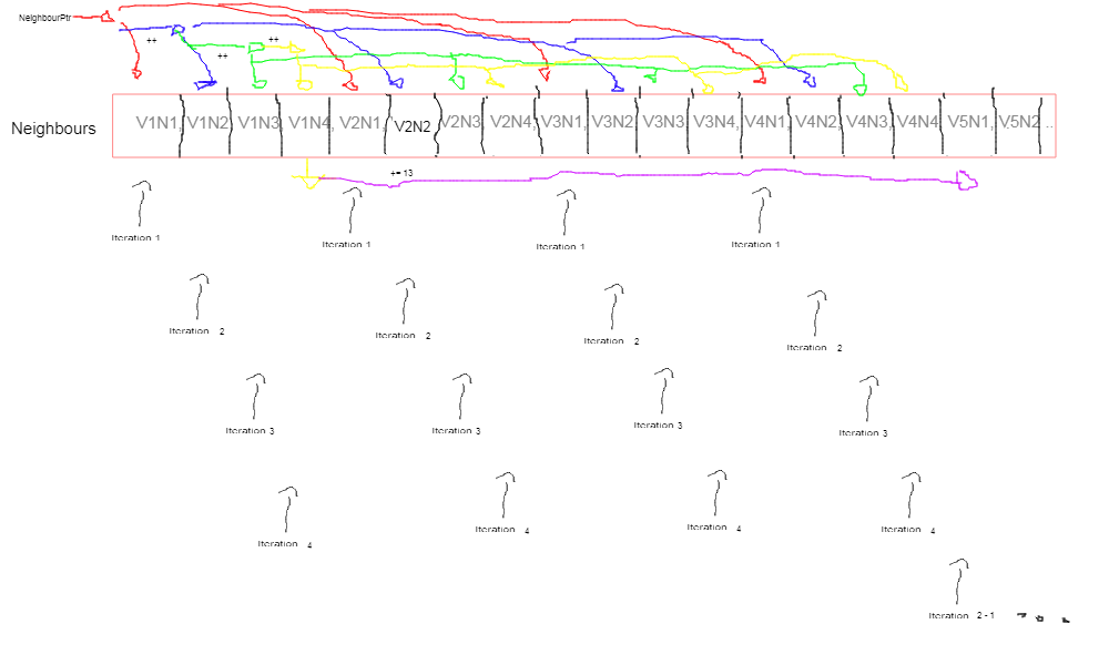
Well, my artistic skills are as bad as always but the point of the image is to show how the pointer changes during the iterations.

We have 3 inner iterations for each main iteration. As you may remember from the previous part this is because we access neighbors in pairs and we always have 4 neighbors to work with.
The pointer starts at the first element of neighbours, the neighbour ID for the first neighbour of the first vertex.
In each iteration, we are going to compute the first pair of neighbors. V1N1, V2N1 … As you can see from the diagram this means we are going to access the element under the pointer and the next 3 elements with an offset of 4 (our count) from each other.
After each iteration, the pointer is increased aligning with the next neighbor ( V1N2, V1N3 … ) and after all the iterations it will end on the fourth neighbor of the current vertex batch ( V1N4, V5N4 … )
With this, we have computed all the neighbors for a vertex batch of 4 vertexes ( 16 elements ) and are on the 4th element of the first vertex of the first batch ( index 3 in the first iteration ). We now need to jump all the computed elements remaining in front of the pointer ( the other 13 indexes ) to find ourselves aligned with the first element of the first vertex of the next vertex batch.

The logic for the delta is similar. We need the delta calculated by the first pair in the first iteration, the second in the second and so on. We’ve previously seen that the deltas are interleaved. This means that the first batch of four has the first delta for vertexes 1-4 and so on. By jumping four double for iteration we go to the next batch of deltas we need for the computations.

Now, let’s try converting some code.

Some practical examples

To start, we have a really simple example as the first part of the main loop, before the inner loop:

// resetting the delta vector
		deltaPtr[0] = 0.0;
		deltaPtr[1] = 0.0;
		deltaPtr[2] = 0.0;

		neighbourIterations = neighbours[vertexIndex].length() - 1;

First of all, our neighbour’s iterations are now fixed. This means we don’t have to find them at runtime anymore as they are constant. We can eliminate that part of the code. The only thing we have to modify, then, is setting the delta to zero. This is easily done, as avx provides a function just for that:

deltaX = _mm256_setzero_pd();
deltaY = _mm256_setzero_pd();
deltaZ = _mm256_setzero_pd();

__m256d smoothedPositionsX = _mm256_load_pd(smoothedX + vertexIndex);
__m256d smoothedPositionsY = _mm256_load_pd(smoothedY + vertexIndex);
__m256d smoothedPositionsZ = _mm256_load_pd(smoothedZ + vertexIndex);

As you can see we are working with 3 (AVX-)vectors for each vector as shown before when talking about SOA. While we are at it we can load the smoothed positions that we have to use multiple times.

Now, this wasn’t much but if we go inside the inner loop we have better things to work with:

tangentPtr[0] = smoothedPositionsPtr[neighbours[vertexIndex][neighbourIndex] * 4] - smoothedPositionsPtr[vertexIndex * 4];
			tangentPtr[1] = smoothedPositionsPtr[neighbours[vertexIndex][neighbourIndex] * 4 + 1] - smoothedPositionsPtr[vertexIndex * 4 + 1];
			tangentPtr[2] = smoothedPositionsPtr[neighbours[vertexIndex][neighbourIndex] * 4 + 2] - smoothedPositionsPtr[vertexIndex * 4 + 2];

			normalPtr[0] = smoothedPositionsPtr[neighbours[vertexIndex][neighbourIndex + 1] * 4] - smoothedPositionsPtr[vertexIndex * 4];
			normalPtr[1] = smoothedPositionsPtr[neighbours[vertexIndex][neighbourIndex + 1] * 4 + 1] - smoothedPositionsPtr[vertexIndex * 4 + 1];
			normalPtr[2] = smoothedPositionsPtr[neighbours[vertexIndex][neighbourIndex + 1] * 4 + 2] - smoothedPositionsPtr[vertexIndex * 4 + 2];

			// Normalizes the two vectors.
			// Vector normalization is calculated as follows:
			// lenght of the vector -> sqrt(x*x + y*y + z*z)
		    // [x, y, z] / length
			length = std::sqrt(tangentPtr[0] * tangentPtr[0] + tangentPtr[1] * tangentPtr[1] + tangentPtr[2] * tangentPtr[2]);

			factor = 1.0 / length;
			tangentPtr[0] *= factor;
			tangentPtr[1] *= factor;
			tangentPtr[2] *= factor;

			length = std::sqrt(normalPtr[0] * normalPtr[0] + normalPtr[1] * normalPtr[1] + normalPtr[2] * normalPtr[2]);

			factor = 1.0 / length;
			normalPtr[0] *= factor;
			normalPtr[1] *= factor;
			normalPtr[2] *= factor;

			// Ensures  axis orthogonality through cross product.
			// Cross product is calculated in the following code as:
			// crossVector = [(y1 * z2 - z1 * y2), (z1 * x2 - x1 * z2), (x1 * y2 - y1 * x2)]
			binormalPtr[0] = tangentPtr[1] * normalPtr[2] - tangentPtr[2] * normalPtr[1];
			binormalPtr[1] = tangentPtr[2] * normalPtr[0] - tangentPtr[0] * normalPtr[2];
			binormalPtr[2] = tangentPtr[0] * normalPtr[1] - tangentPtr[1] * normalPtr[0];

			normalPtr[0] = tangentPtr[1] * binormalPtr[2] - tangentPtr[2] * binormalPtr[1];
			normalPtr[1] = tangentPtr[2] * binormalPtr[0] - tangentPtr[0] * binormalPtr[2];
			normalPtr[2] = tangentPtr[0] * binormalPtr[1] - tangentPtr[1] * binormalPtr[0];

All of this too will be pretty straightforward. This will be true for mostly anything I had to vectorize on this code. There may be some cool trick to speed some things up but a simple translation does not require much apart from the basic functions as this code lends itself to a, mostly, 1:1 conversion. Better yet, having gone the SOA form way we find ourselves, yet again, in a great position as we don’t have to shuffle or permute the vectors to compute some of our operations.

Let’s start. First, we have to load our neighbors and compute the displacement between our vertexes and them.

__m256d neighboursPositionX = _mm256_setr_pd(smoothedX[neighbourPtr[0]], smoothedX[neighbourPtr[0 + 4]], smoothedX[neighbourPtr[0 + 8]], smoothedX[neighbourPtr[0 + 12]]);
__m256d neighboursPositionY = _mm256_setr_pd(smoothedY[neighbourPtr[0]], smoothedY[neighbourPtr[0 + 4]], smoothedY[neighbourPtr[0 + 8]], smoothedY[neighbourPtr[0 + 12]]);
__m256d neighboursPositionZ = _mm256_setr_pd(smoothedZ[neighbourPtr[0]], smoothedZ[neighbourPtr[0 + 4]], smoothedZ[neighbourPtr[0 + 8]], smoothedZ[neighbourPtr[0 + 12]]);

As said before, we are going to access the neighbors 4 at once with an offset of 4. Instead of loading them, then, we get to set them directly.

The r in setr stands for reverse ( I think ). While _mm256_set_pd will set the arguments passed right to left starting at the least significant bit, _mm256_setr_pd will set them left to right starting at the least significant bit. Basically, with set, the leftmost argument is actually the last element of the vector ( residing in the most significant X bit of it ) while with setr we get them with the order we visually see them and might expect them to be positioned.

Since we are working with pairs we will load ( after some computations ) another set of neighbors starting at index 1. But before that we should work a bit on our vector:

tangentPtr[0] = smoothedPositionsPtr[neighbours[vertexIndex][neighbourIndex] * 4] - smoothedPositionsPtr[vertexIndex * 4];
tangentPtr[1] = smoothedPositionsPtr[neighbours[vertexIndex][neighbourIndex] * 4 + 1] - smoothedPositionsPtr[vertexIndex * 4 + 1];
tangentPtr[2] = smoothedPositionsPtr[neighbours[vertexIndex][neighbourIndex] * 4 + 2] - smoothedPositionsPtr[vertexIndex * 4 + 2];

length = std::sqrt(tangentPtr[0] * tangentPtr[0] + tangentPtr[1] * tangentPtr[1] + tangentPtr[2] * tangentPtr[2]);

factor = 1.0 / length;
tangentPtr[0] *= factor;
tangentPtr[1] *= factor;
tangentPtr[2] *= factor;

Again, this is a mostly 1:1 conversion. First, we have our smoothedPositions ( that we found before ) and our neighbors smoothed positions. We have to subtract them and as you know this is nothing more than a simple function away from us.

__m256d tangentX = _mm256_sub_pd(neighboursPositionX, smoothedPositionsX);
__m256d tangentY = _mm256_sub_pd(neighboursPositionY, smoothedPositionsY);
__m256d tangentZ = _mm256_sub_pd(neighboursPositionZ, smoothedPositionsZ);

We do it component wise like we mostly did it before, but now we are working with more data each time. The normalization is a bit cuter but nonetheless simple.

__m256d length = _mm256_sqrt_pd(_mm256_add_pd(_mm256_mul_pd(tangentZ, tangentZ), _mm256_add_pd(_mm256_mul_pd(tangentX, tangentX), _mm256_mul_pd(tangentY, tangentY))));
__m256d factor = _mm256_div_pd(_mm256_set1_pd(1.0), length);

tangentX = _mm256_mul_pd(tangentX, factor);
tangentY = _mm256_mul_pd(tangentY, factor);
tangentZ = _mm256_mul_pd(tangentZ, factor);

Having access to the component separately helps use here ( and in mostly any operation on vectors we do ) by simplifying our code a lot. The only new thing here is _mm256_sqrt_pd which, as you probably guessed, computes the square root of each element of the vector.

We will be doing the same things for most of the code so I won’t cover it all. As you can see, most of the work for a basic conversion was already in place by structuring our code adequately.

Wrapping it up and what I’m doing right now

There were some more things I would have liked to show in this post. Most of these can be found in the code. I found out that writing a post with only about an hour a day of writing ( the train time I have in the morning ) greatly decreases the speed at which I can write. Just like with code, losing your train of thoughts has a terrible productivity impact.

Looking forward, I finally got somewhat accustomized to my new time’s constraints and am squeezing the most out of the small free time I have.

Regarding the deltaMush, The next step is to go and parallelize our deformer.

Now, I’ve used Maya Threads in the past but for this project, I absolutely want to try out Intel’s TBB. Furthermore, I’m studying some theory and general knowledge about parallel programming to approach the parallelization of this project with a little more consciousness. This obviously means that some time will pass before the next version of the code. I’m thinking about doing more than one parallel version as I’m really liking the differences in Threading libraries and would like to try more than one.

This is something I’m still pondering about as the time is really strict and I should not use too much time on a single thing ( especially since I should be working on more (entry-level ) work-appetible projects ( maybe an autorigger or something ) if I don’t want to be stuck in my current work ).

For this same reason, I will probably spend less time on micro-optimizations and tests ( as was already done for this part of the code ). For how unfortunate and joy-depriving that is.

In the meantime, I am actually following some more projects and studies when I can’t use my laptop. One of the things that, currently, is giving me happiness is the study of the Factor programming language. I fell in love with it while reading Seven More Languages in Seven Weeks and could not stop myself from studying it.

My allotted time for it is really small, unfortunately, and consists of only my lunch break at work. Nonetheless, I’m making small but surely steps and would like to write about this beautiful language, which is only the third language that has made me feel so lovestruck ( after Haskell [ which I will one day learn decently ] and pure C which was my first love ), sometimes.

Another thing I got pretty interested in is competitive programming. I’m using it as a study subject for when I can’t use my laptop ( as I can do it on my phone without too many problems ) and am solving exercise problems in both C++ and Factor. It’s crazy how many interesting things I’m learning about the STL ( or the standard Factor vocabularies ) that I didn’t know. I may decide to write something about this too.

I’m trying to further my functional programming understanding as it is a paradigm I really love.

If I can squeeze a bit of time from my sleep ( For now it seems impossible as I’m already sleeping the least my body is able to tolerate ) I’d like to start studying assembly again as I was loving it before starting to work.

Lastly, I’m learning a lot at work. Most of it is web-based as I’m working as a back-end developer. I’m really grateful for all the things I’m being taught or am discovering while working.

PHP is not that bad of a language I once thought ( it has its bads, tough, but it is really really suited to what we do at work ).

Nonetheless, I must say I still feel extraneous to the programming I do at work and can’t get myself to get as excited as when I study other programming topics. I don’t think I will ever write something about it on this blog. May do a story post on my first work-experience but I’ll see.

This is more than enough chit-chat. If you’ve come this far I hope that this article was useful to you and hope to see you next time.

https://www.codeproject.com/Articles/874396/Crunching-Numbers-with-AVX-and-AVX https://www.agner.org/optimize/ ( It should be read entirely but regarding vector operations look at the first manual and at agner’s library ) https://software.intel.com/sites/landingpage/IntrinsicsGuide/ http://www.posix.nl/linuxassembly/nasmdochtml/nasmdoca.html https://deplinenoise.wordpress.com/2015/03/06/slides-simd-at-insomniac-games-gdc-2015/ https://lxjk.github.io/2017/09/03/Fast-4x4-Matrix-Inverse-with-SSE-SIMD-Explained.html